TL;DR
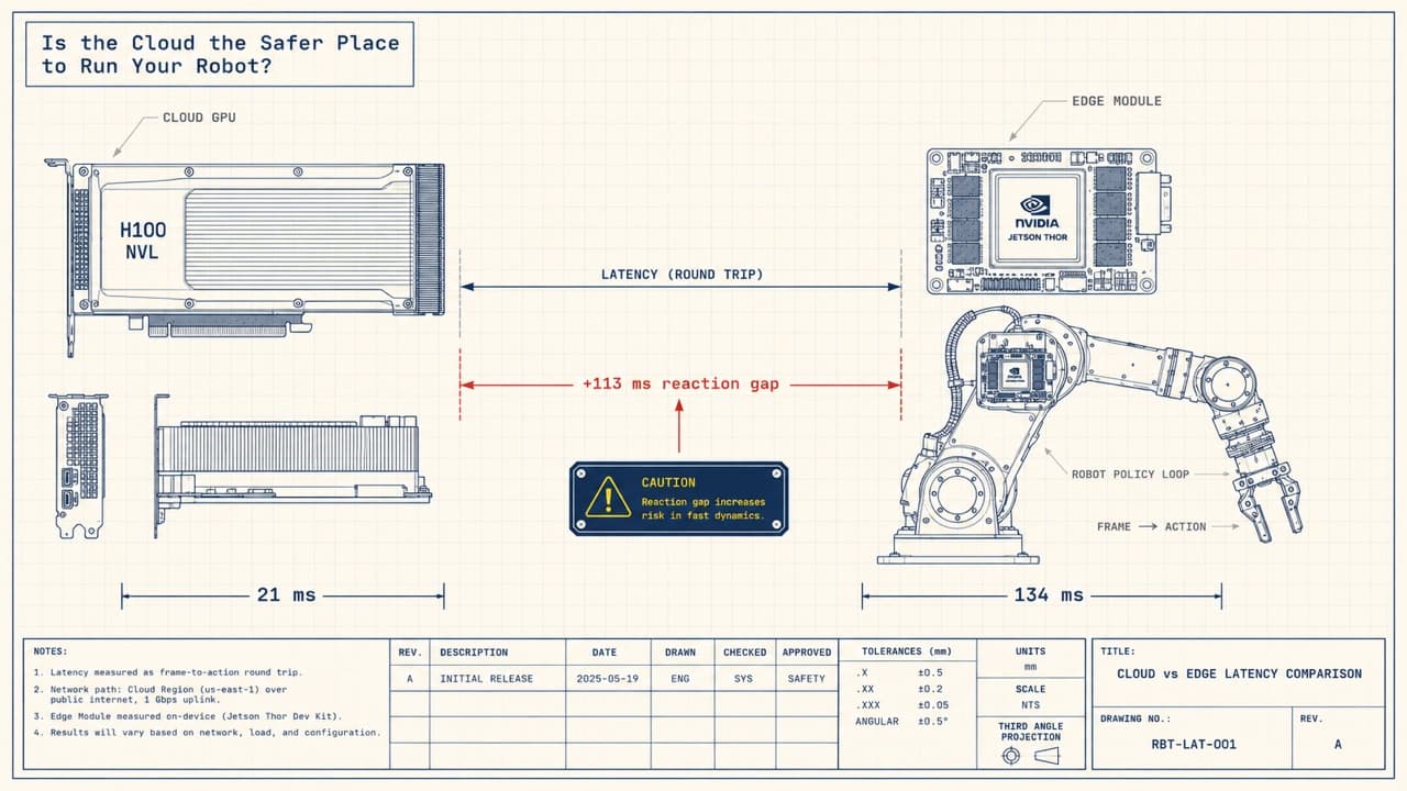
- Unquantized, the same robot policy runs about 6× faster in the cloud than on the edge: Pi0.5 is 21 ms on a cloud GH200 (H100-class), 134 ms on a Jetson Thor.
- The optimization behind it is one CUDA graph over the whole forward pass. It barely helps the edge, which is already saturated on its matrix multiplies, so the gap is real, not a tuning artifact.
- That makes the cloud a real candidate where reaction speed is the safety property that matters, at least until quantization narrows the edge (next post).
The question we keep getting
Why robotics defaults to the edge, the question teams actually ask us, and what this post measures.
In the LLM world, where the model runs was settled early: nearly every model you use lives in a datacenter and reaches you through a web app, because users can wait a second or more for an answer, and a dropped connection is a spinner, not a disaster. A robot is not like that. It may need to be ready all the time and react in milliseconds. So robotics policies default to the edge.
People ask us at Haptic whether it even makes sense to deploy a robotics model to the cloud, "given the physics of latency." Or more bluntly: "What's better for me, buying a $3,000 Jetson chip and distilling a model so it runs locally... or renting a beefy cloud GPU and running a bigger model?" Finetuning, latency, and reliability all play in, so we wrote this post to share how we think about the dance between edge and cloud.
This first post measures one thing: how fast the same policy runs in the cloud versus on the robot. The next one looks at what optimizing the edge can claw back.
The edge-vs-cloud decision
The questions that decide it before you run a single benchmark: the speed budget, where the time goes, and whether the network can carry it.
If you already know control loops, VLA inference, and frame-to-action budgets, skip to how a VLA policy runs.
Deciding edge vs cloud for your robot comes down to a handful of questions:
- How fast does it need to be? The task sets a floor on the policy loop rate, and that floor is the budget everything else fits inside.
- Where does the time go? Frame-to-action latency is a round trip with four legs, and only one of them is the model.
- Can the network carry it? Camera observations flow upstream, the direction most links are thinnest, and the link is judged on drops, not just throughput.
- What does each side give up? Compute, reliability, model ceiling, power: the trade in one table.
One constraint frames all of them: physical AI is a co-design of hardware, software, and model. A mobile robot's battery bounds its power, the power bounds the chip it can carry, and the chip bounds the model it can run. A datacenter has no such chain.
How fast does it need to be?
As fast as the task demands: tens of Hz for reactive work, under 1 Hz for replanning. But first, which loop are we even talking about? A robot runs a stack of them, and they do not all live in the same place:
- Servo loops. Torque and joint control, 1 kHz and up, on the motor drives and real-time controller. These stay on the robot no matter what; nobody proposes putting them through a datacenter.
- The execution loop. A real-time controller plays out the policy's current action chunk at, say, 50 Hz. Also stays on the robot.
- The policy loop. A model turns camera frames into actions. This is the contested loop, and the one this post is about.
What the policy loop has to achieve depends on the task:
| Task | Policy loop rate | Frame-to-action budget |
|---|---|---|
| Flinch from a hand, catch a slipping grasp | 10-30 Hz | 30-100 ms |
| Visual servoing, moving-target tracking | 10-30 Hz | 30-100 ms |
| Pick, place, deliberate assembly | 2-10 Hz | 100-500 ms |
| Task-level replanning ("now do the next part") | <1 Hz | seconds |
The budget is concrete: an arm moving at 1 m/s travels 10 cm for every 100 ms it is blind to a new frame.
Chunking buys smoothness, not reactivity. The 50 Hz playout looks continuous, but the policy loop still closes at only 1 to 10 Hz, and the robot responds only to what happened before the frame its current chunk was computed from. Frame-to-action latency is the reactivity number even when the motion looks smooth.
Where does the time go?
Mostly into inference; the network adds tens of milliseconds on either side of it. The frame-to-action round trip has four legs:
- Capture and encode. A camera frame is grabbed and compressed to JPEG on the robot. ~1-5 ms.
- Upload. The ~50 KB observation crosses the network to a nearby datacenter. ~10-30 ms.
- Inference. The GPU runs the forward pass and produces an action chunk. The contested leg, and the one we measure on both targets below.
- Download. The chunk, a few KB, comes home and the arm moves. ~5-15 ms.
Frame-to-action latency is the sum of all four, and it has to fit inside the budget column above. On the edge, steps 1, 2, and 4 collapse to nearly zero: the frame never leaves the robot. The cloud's bet is that step 3 is enough faster to pay for the trip and still get the action back sooner.
Can the network carry it?
The bandwidth you need is modest, but it points the wrong way for most links. A robot uploads an image and gets a tiny action chunk back, so its upload demand is 10 to 100× its download demand. Concretely, a Pi0.5 observation is three 224×224 RGB cameras, about 450 KB raw or ~50 KB JPEG per inference going up, while the action chunk coming down is a few KB. That is the reverse of consumer connectivity, which is provisioned fat-down, thin-up.
To hold 10 Hz you need roughly 4 Mbps of sustained uplink compressed, ~36 Mbps raw. A wired factory network clears that easily; Wi-Fi and cellular can do it, but they have to prove it on jitter and drop rate, not just average throughput, because a late frame is a stale action and a dropped link is a frozen arm.
What each side gives up
| Edge (Thor on the arm) | Cloud (H100) | |
|---|---|---|
| Inference speed | slower, compute-bound | faster, this post's subject |
| Link drops | keeps working | freezes mid-motion |
| Network in the loop | no | every cycle |
| Model ceiling | 128 GB, fixed at purchase | whatever you rent |
| Upgrades | replace hardware | redeploy |
| Power | the battery's problem | the datacenter's problem |
| Cost shape | capex, per robot | opex, shareable |
So the choice comes down to two measurable things: how fast the robot reacts, and what happens when the link drops. Most teams pick edge for the second and never measure the first. That measurement is the rest of this post.
How the policy actually runs
A flow-matching VLA in two phases, and the one quirk of single-frame inference that makes it slow in a way we can fix.
If you already know how prefill and denoise work and why single-frame inference is launch-bound, skip to one graph instead of thousands of launches.
What the policy computes
- Prefill, once per frame. The vision tower and language backbone encode the camera images and text prompt into a key/value cache that the denoise phase reuses. This is the big, timestep-independent part, a 3B PaliGemma for Pi0.5, a 5B vision-language stack for MolmoAct2.
- Denoise, a few times per frame. A small action expert starts from noise and takes a handful of steps, attending to that cached prefix each step, until it emits an action chunk: the next short slice of motion the robot executes.
Why it's slow in a way we can fix
A robot processes one observation at a time, so there is no batch to amortize over. At batch=1 the matrix multiplies are small, and on a fast GPU each one finishes almost as soon as it starts. The wall-clock cost is not the arithmetic. It is getting thousands of tiny kernels (the individual GPU operations) onto the card one at a time, each waiting on the CPU to launch it. That is the launch-bound regime: the GPU sits idle between launches instead of staying busy. It is what CUDA graphs exist for.
One graph instead of thousands of launches
The whole speedup is a single CUDA graph over the forward pass. Here's the catch that makes it hard, and how we cleared it on all four families.
Since the bottleneck is launch overhead and not arithmetic, we can attack it with a CUDA graph: record the kernel sequence once and replay it with a single launch, no per-kernel CPU overhead.
There is a catch. Capture requires fixed tensor shapes, fixed memory addresses, and no operation that copies between host and device or syncs the two. Break one rule and it aborts. The denoise phase already obeys these rules, fixed shapes by construction, a clean function of (prefix, noise, timesteps), so it was already graphed. The prefill phase is the problem, and therefore the opportunity: it's the only phase left to capture, and it breaks the rules by running small host-to-device operations that are harmless in eager mode (PyTorch one op at a time) but fatal during capture. Getting prefill to comply, across all four model families, is the rest of this section.
The three things capture can't tolerate
All four families broke capture the same way, with different specifics. Each time, the problem was a host-to-device or data-dependent op, and each fix produces output byte-for-byte identical to the original:
| Capture-killer | Why capture dies | The fix |
|---|---|---|
torch.tensor([0, 0, 1, ...], device="cuda"), a mask built from a Python list | builds on the host, copies to device every call | precompute it once into a buffer |
torch.full((), -inf), a mask-fill scalar made on device each call | a fresh host-to-device op every call | cache the scalar |
| a slice with a boolean mask | data-dependent output shape, the single most common killer | gather at fixed, cached indices |
The worst offender, in full
The boolean-mask slice showed up three times, so it is worth seeing whole. GR00T's Eagle backbone scatters image features into the token stream with flat[is_image_patch] = image_features. The boolean index calls nonzero internally, its output shape depends on the data, and capture dies. The fix runs that nonzero once eagerly, caches the indices, and uses index_copy_ at the image-token positions: the same operation, the same bytes.
idx = self._image_token_idx(is_image_patch)   # nonzero once, eager, then cached
flat = flat.index_copy(0, idx, image_features)
MolmoAct2 had the nastiest version, buried in the vision pooling (pooled.view(-1, d)[valid_token.flatten()]): same boolean-index, same fix. It also drew its noise inside the forward pass and handed the prefill KV cache to the denoise loop through a cache object. Folding it into one graph meant turning the noise into an explicit input and giving the cache a clone() so the graph could return it: five edits on the most complex family.
Proving the numbers never moved
Every one of these edits is checked bit-identical, the same discipline as the format-conversion work. The graphed output equals the un-graphed output to the last bit, max difference 0.000e+00, because a replay runs the identical kernels. A golden gate, a saved reference output the new code is diffed against, catches any fix that quietly changes the output.
In the cloud: 3-7×
Same policy, one denoise step, on a cloud H100. The graph pays off.
GH200, which is H100-class, bf16, one denoise step (the deployment target, the single step our SnapFlow distillation is landing next). Eager is the model running normally; full-graph is the whole forward captured once and replayed.
| Family | eager | full-graph | speedup | parity vs eager |
|---|---|---|---|---|
| Pi0.5 | 88 ms | 21.5 ms | 4.0× | 0.000e+00 |
| SmolVLA | 62 ms | 9.1 ms | 6.8× | 0.000e+00 |
| GR00T | 39 ms | 7.2 ms | 5.4× | 0.000e+00 |
| MolmoAct2 | 143 ms | 48 ms | 3.0× | 0.000e+00 |
A few honest notes. SmolVLA wins most because it is the smallest backbone, so it is the most launch-bound: the least arithmetic per launch. MolmoAct2 wins least at 3.0× because at 5B params it is already partway into compute-bound even on an H100, its arithmetic finally large enough to matter. That spread, from 6.8× down to 3.0× as the model grows, previews the edge result: the larger the model, the more of its time already goes to arithmetic rather than launch overhead, and the less a CUDA graph can give back.
On the robot: almost nothing
We synced the same code to the Jetson Thor on the arm and ran it. Four milliseconds.
The Thor is the point of all of this. It is the GPU bolted to the arm. So we synced the same branch, the same checkpoints, the same benchmark, and ran it. bf16, one step:
| Family | eager | full-graph | speedup |
|---|---|---|---|
| Pi0.5 | 138 ms | 134 ms | 1.0× |
| SmolVLA | 37 ms | 27 ms | 1.4× |
| GR00T | 42 ms | 36 ms | 1.2× |
| MolmoAct2 | 193 ms | 174 ms | 1.1× |
Still bit-identical, still graphed, and barely faster. Pi0.5 in particular went from 138 ms to 134 ms, four milliseconds on a thing that was four times faster on the H100. The reasonable first reaction, and the one we had, is to distrust the measurement. Is it replaying the graph, or silently falling back and reporting the same number twice?
We didn't believe it either
The graph is really replaying; it just has nothing to do on the Thor. One number explains both machines: how much of the time the GPU is busy.
The graph really is replaying, not silently falling back to eager: the profiler shows one cudaGraphLaunch per inference where eager fires about 6,400 separate launches, the runner reports replay mode, and the output is bit-identical. The graph is real. It just has nothing to do on the Thor.
The reason is one number, and it is the same number on both machines: how much of the wall-clock time the GPU is busy.
pi0.5, 1 step, bf16, eager:
  H100/GH200:  wall 84 ms  | GPU busy  47%   <- idle half the time = launch-bound
  Jetson Thor: wall 136 ms | GPU busy ~100% <- saturated on GEMMs = compute-bound
(These wall times are from a profiler run, a touch off the benchmark tables above; the figure that matters here is GPU-busy.) On the H100, at batch=1, the GPU is idle 53% of the time. It finishes each small matrix multiply and then waits for the CPU to hand it the next one. That idle gap is pure launch overhead, and it is the ~63 ms a CUDA graph removes (84 ms to 21 ms, the GPU now 92% busy). On the Thor the same matrix multiplies take long enough that the GPU is never waiting: it is busy the whole time running them. The top kernels on both machines are the same, aten::mm and the cuBLAS GEMM kernels, but on the H100 they are a small share of a launch-dominated wall, and on the Thor they are the wall. There are only a couple of ms of launch overhead on the Thor to remove, so that is all the graph removes.
A CUDA graph looks like an edge optimization, cut the CPU overhead, help the small device, but here it is the opposite: an optimization for datacenter GPUs. It helps most where you need it least, on the big cloud card with throughput to spare, and least where the latency hurts most, on the small edge card that is already maxed out. That is the technical fact. The interesting part is what it implies once you put the two absolute numbers next to each other.
So is the cloud safer?
Add up the round trip and the cloud still reaches the action first. Then the two things that decide whether that holds on a real robot.
The measurement
Add up the round-trip legs from earlier:
- Capture and encode the frame on the robot: 1-5 ms
- Upload the observation: 10-30 ms
- Inference on the cloud GPU: 21.5 ms
- Download the action chunk: 5-15 ms
That's roughly 38 ms best case, 72 ms worst, frame to action with the network fully charged. The Thor, paying for none of those legs but inference, is 134 ms. Even at the top of the cloud's range, every network leg included, it reaches the action nearly twice as fast as the edge does with no round trip at all. The round trip was supposed to be the cloud's disqualifier; pay it in full and the cloud still reaches the action first.
The last section is why that gap is trustworthy rather than a tuning fluke: the cloud was slow for a reason a CUDA graph removed, the edge for one it can't. Idle launch-bound time is free to remove; the arithmetic the Thor is saturated on is not. The cloud had headroom the edge structurally lacks, so the lead survives equal effort on both sides.
For the loops where reaction time is the point, visual servoing, tracking a moving target, closing a grasp under deliberate control, that makes the cloud faster at the thing the edge was supposed to own, not a compromise you accept for a bigger model.
What bends it in deployment
Read these as early numbers, not a guarantee. Two things decide whether the margin holds on a real robot.
The first is jitter. The Thor's 134 ms is deterministic, the same every cycle, while the cloud's 38-72 ms is a mean with a tail, and a reactive loop is judged on its worst frame, not its average. One congested upload on factory Wi-Fi and that 72 ms becomes the number that misses the slipping part.
The second is the batch=1 assumption baked into the inference figure, which measures one robot to a card. Share that card across robots and queueing can creep back into the tail. The clean best case is real; the deployed distribution is what you measure on your own network before you trust it.
The edge's answer: quantization
The Thor is compute-bound, so its lever is cheaper matrix multiplies. How far FP8 and NVFP4 close the gap, and the trap that fakes it.
The right kind of cheaper
The Thor is compute-bound, so its lever is the one the cloud doesn't have: make the matrix multiplies themselves cheaper. The catch is that "cheaper" has to mean the format the tensor cores compute in, not just the precision the weights sit in at rest.
That distinction kills the obvious move. Weight-only 4-bit, the popular AWQ and GPTQ path, shrinks the weights you fetch but keeps the arithmetic in fp16. On a memory-bound LLM decode that's a real win. On the Thor's compute-bound prefill it does close to nothing, because fetching weights was never the bottleneck. Easy to reach for, wrong tool here.
The formats that earn their keep on a Blackwell Thor are FP8 and, below it, NVFP4, a 4-bit format with a per-16-element scale. By NVIDIA's published tensor-core specs, FP8 runs roughly 2× bf16 and dense FP4 roughly 2× FP8 again, and that's speed off the wall, not just off disk.
The measured result
We are not theorizing. NVIDIA's Jetson AI Lab tutorial deploys the OpenPi Pi0.5 policy on a Jetson AGX Thor and benchmarks it end to end: 162.6 ms in PyTorch BF16, ~94 ms quantized to FP8 plus NVFP4 through TensorRT. That's 1.73×, at 0.9956 cosine similarity against the bf16 output, close enough to call the quantized model faithful. Different stack from our 134 ms run, so it's the speedup that transfers, not the wall-clock: apply 1.73× to our number and the edge closes from 134 ms to roughly 80 ms. It narrows the gap, it doesn't erase it, the cloud's 38-72 ms still sits under that, and the open question is what quantization costs in task success on a real robot, worth measuring, not asserting.
A trap when you reproduce this
One trap would quietly invalidate the whole comparison. On the Thor's sm110 silicon the TensorRT builder will accept an FP8 or FP4 flag and silently build an FP32 engine: no warning, larger file, float outputs. You catch it only by checking that the engine shrank and the cosine similarity moved. The lesson from the bit-identical gates earlier: verify the number, don't trust the flag.
Run it on both
There's no universal winner. A decision tree for where your policy should live, by link reliability and reaction budget.
The point is not to crown a winner. After optimizing both ends the cloud is faster, often by enough to matter. But "faster" only turns into "safer" under conditions you can check up front. Here is the decision the way we actually walk it with a robot in front of us:
Where should this policy run?

1. Can the robot tolerate the link dropping mid-motion?
   No   ->  Edge. A frozen arm is the failure you can't accept, and no
            latency win buys it back. Stop here.
   Yes  ->  keep going.

2. Is the loop reaction-bound? (flinching, catching a slip, visual
   servoing: a 30-100 ms frame-to-action budget)
   No   ->  Either works. Decide on the model and how you'd rather pay:
            edge is simplest and bought once; cloud lets you run a model
            past the Thor's 128 GB and upgrade without swapping hardware.
   Yes  ->  keep going.

3. Does your network hold a low-jitter round trip inside that budget?
   Yes  ->  Cloud. After optimizing both ends it reaches the action
            first, ~38-72 ms against the Thor's 134 ms, round trip and all.
   No   ->  Edge. A deterministic 134 ms beats a faster average with a
            tail that misses the frame that mattered.
So the title answers itself, with conditions attached: the cloud is the safer place to run your robot when the link is reliable and reaction time is the risk, and the edge is safer the moment either of those flips. Quantization (the next post) moves the third branch, not the first.
If you are running a Pi0.5, GR00T, SmolVLA, or MolmoAct2 policy and trying to decide where it should live, the cloud or the Thor on the arm, we will run it on both and hand you the per-family latency and parity numbers for your robot. Talk to us.
What's next:
- Quantize the prefill matrix multiplies to FP8, then NVFP4 where it pays, through NVIDIA's Model Optimizer to a verified TensorRT engine, and report per-family Thor latency and the task-success cost the way we reported the graph numbers here.
- Keep the graph. It is free and bit-identical, it helps every cloud target, and on the edge it composes with quantization rather than competing with it: a quantized engine still benefits from one launch instead of thousands.
- Land the SnapFlow single-step distillation into the same measurement, so the denoise loop is one step and the prefill is unambiguously the bottleneck the quantization is aimed at.
The latency numbers are CUDA-event-timed on a GH200 and a Jetson Thor, bf16, one denoise step, parity checked bit-identical against the un-graphed model each run.