LIBERO-Spatial task 0, side by side: Pi0.5 FT teacher (4.14 B params, 8.3 GB) on the left, V8-trim + INT8 student (2.31 B params, 2.85 GB) on the right. Same task, ~3× smaller model.
Shrinking Pi0.5 by 2.9× on disk and 2.8× faster. The paper gives you the recipe. We're sharing what it costs to actually run that recipe end-to-end.
TL;DR
- Shrinking robotics models makes them faster and lets them run on cheaper, lower-power hardware.
- We shrank Pi0.5 using two techniques: layer pruning and INT8 quantization.
- End result: 3.0× smaller in memory, 2.9× smaller on disk, 2.8× faster, with approximately the same task quality (LIBERO-Spatial, simulation).
- The recipe is in the paper. The pipeline tax (six silent failures, ~4 days of compute lost) is what makes this hard in production. That's the slot we're filling.
- We are onboarding more design partners. Talk to us if you want to:
- shrink a VLA to fit your robot's actual compute,
- turn a generalist model into a task specialist for production, or
- stay on the frontier automatically as new SOTA VLAs ship.
Context
Why shrinking models matters, how it connects to last week, and helpful context.
Why shrinking models matters
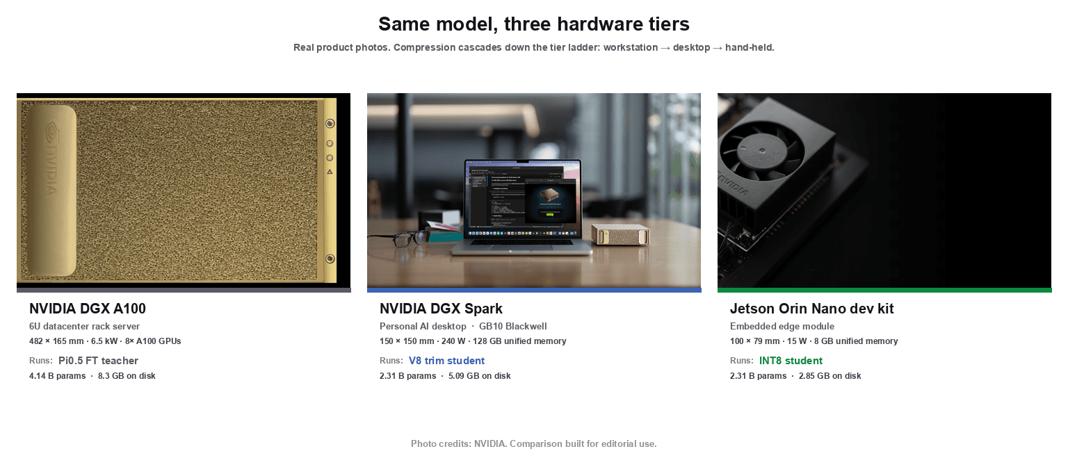
Robots are sensitive to model size. An LLM that's too big just costs more to serve; you rent a bigger GPU. A robot doesn't have that option. It has a fixed chassis, a fixed battery, a fixed thermal envelope. So when the model doesn't fit or is too slow to be usable, you have three choices:
- Don't ship.
- Redesign the robot around the model.
- Shrink the model to fit the robot.
This post is about option 3.
Last week: time. This week: size.
Last week was about time: making inference faster. We used SnapFlow, a published self-distillation recipe, to teach Pi0.5 to do in 1 step what used to take 10. (Full writeup.)
So this week's question was simple: can we make the backbone itself smaller?
Pi0.5 is built from three transformer stacks: 18 layers in the language model, 18 in the action expert, and 27 in the vision tower. Two ways to shrink it, and they stack: cut layers (pruning), and use fewer bits per remaining weight (quantization).
The pruning story
Three sections on how we trimmed Pi0.5 from 4.14B to 2.31B parameters: getting stuck, finding the bug, and breaking through.
The recipe we wanted to replicate
For pruning, the most relevant prior art is Shallow-π (Jeon et al., January 2026, Samsung Research). The paper takes a flow-based VLA much like Pi0.5, prunes the language model and action expert from 18 layers to 6, and recovers 94.6% on LIBERO-Spatial through knowledge distillation, within 1% of the unpruned teacher.
The published recipe has three loss terms:
L_task: the standard flow-matching objective the model was originally trained with.L_kd: the student's velocity prediction matches a frozen teacher's velocity at the same noise level.L_attn: the student's middle-layer cross-attention matches the teacher's, on the action-token to vision-language-token submatrix only.
That third term (L_attn) is what the paper's ablation singles out as essential. Without it, the 6-layer student lands at 93.9%. With it, 94.6%. Small gap, but it's the gap between “this works” and “this doesn't”, and we'll spend most of the next two sections fighting it.
We re-implemented all three and started training. So far, so good.
Three days of 70 / 30%
This is where we got stuck for 3 days.
Every variant we tried plateaued at the same ceiling: 70% accuracy at 1-NFE. 30% at 10-NFE.
| Variant | What changed | Result |
|---|---|---|
| V2 | L_task + L_kd only, no L_attn | ~70% / 30% |
| V3 | Full Shallow-π recipe at 8x A100 | Diverged (gradient norm 1e10 at step 3000) |
| V4 | log_softmax fix for numerical stability | Still diverged |
| V5 | Lower L_attn weight | ~70% / 30% |
| V6 | Linear L_attn warmup over 3000 steps | Diverged at warmup completion |
| V7 | Reverse KL (mode-seeking instead of mean-seeking) | Plateaued at 70%, gradient clip saturated |
And the wrong direction: 10 passes was worse than 1 pass. Normally you work to reduce passes while keeping accuracy the same; here the model was getting worse with more passes, which signals something is broken at the loss level. Three days went by. Whatever was wrong, it wasn't in the knobs we were turning.
Reading the footnotes
After 3 days, after running every variation we could think of and being firmly stuck, we did what we should have done on day one: read the references.
Shallow-π's L_attn term is, in the paper's words, “inspired by Align-KD.” Align-KD (Feng et al., CVPR 2025) is a knowledge-distillation method for mobile vision-language models. Their loss formula, Equation 1, is:
L_attn = MSE(P_attn(A_teacher), A_student)Or more simply stated:
L_attn = MSE(teacher's attention, student's attention)Their formula uses MSE, not KL (as we had been using). In short: Shallow-π wrote KL in the paper, but it looks like they actually ran MSE in their codebase. We can't tell what they actually ran to get their numbers. But Align-KD, the paper they cite, is clear: use MSE. That was the moment it clicked.
Why does that matter? Attention values are probabilities, so MSE on them is bounded in [0, 1]. KL has no such ceiling: when the teacher is confident on a token the student got near-zero on, KL's log(near-zero) term goes to negative infinity, the loss blows up, and gradients with it. This is a known KL-distillation failure mode with a known fix: switch to MSE.
We changed one line, replaced KL with MSE on the attention values, re-ran the smoke test. It worked.
Breaking the ceiling
V8 was the run after the MSE fix.
We launched a 5,000-step smoke test (a short low-cost run to check if anything works at all). Loss dropped smoothly from 1.12 to 0.081. Gradient norm stayed below 1.0 the entire time. No explosions. No saturation. We ran it to completion, held our breath, and evaluated against 200 episodes of LIBERO-Spatial.
81.5% at 1-NFE. 59.0% at 10-NFE.
The ceiling broke. The 1-NFE / 10-NFE asymmetry was still there, but the model was actually learning.
We trained out to 15k and then 30k steps to see how far it would go.
| Step | 1-NFE | 10-NFE |
|---|---|---|
| 5k | 81.5% | 59.0% |
| 10k | 88.0% | 74.5% |
| 15k | 91.0% | 83.5% |
| 25k | 90.0% | 86.0% |
| 30k | 88.0% | 86.5% |
The 1-NFE / 10-NFE asymmetry shrank from 22 points at 5k down to 1.5 by 30k (early in training the pruned model accumulates errors across partial denoising steps; by 30k it has learned to refine). At 30k the 10-NFE accuracy is about 7 points below the unpruned teacher. That's a real cost. We're not going to pretend otherwise. The week's question was whether size compression is viable on this model, not whether it's free. It's viable, with a known accuracy delta.
Now that we had successfully pruned layers, we moved on to the next technique: quantization.
The quantization story
One section on how we halved every remaining weight from 16 bits to 8, in three lines of code.
Going to INT8
Pruning took three days, but quantization took an afternoon.
With the trimmed student in hand at 2.31 B parameters and 86.5% accuracy, we turned to quantization. The goal was simple: shrink each remaining weight from 16 bits to 8.
We used torchao's Int8WeightOnlyConfig, the PyTorch team's quantization library. The conversion is three lines:
from torchao.quantization import quantize_, Int8WeightOnlyConfig

policy = load_pi05_policy(checkpoint_path, dtype=torch.bfloat16)
quantize_(policy.model, Int8WeightOnlyConfig())
torch.save(policy.model.state_dict(), "model.pt")
The library walks through the model and replaces every weight with an 8-bit integer version, plus a small scaling factor per output channel to keep the precision close to the original. From the outside, the model behaves identically. Internally, it streams half as much data per forward pass.
We chose weight-only quantization (rather than the more aggressive W8A8) because it's the conservative starting point: weights are quantized but activations stay at bf16. The math still runs at bf16 precision, so latency wins are limited to memory streaming, not the matmul itself. The full INT8 GEMM win comes from W8A8 plus calibration ( SmoothQuant, LLM.int8()), which we'll graduate to next. Ours held on accuracy, so we shipped weight-only for week 2.
Results. Same 200-episode LIBERO-Spatial eval as the trim work. Here's how int8wo compares against the bf16 V8 student:
| bf16 V8 30k | int8wo V8 30k | delta | |
|---|---|---|---|
| On-disk | 5.09 GB | 2.85 GB | -44% |
| Runtime memory peak | 9.4 GB | 3.1 GB | -67% |
| A100 1-NFE accuracy | 88.0% | 91.5% | within variance |
| A100 10-NFE accuracy | 86.5% | 85.5% | within variance |
| Spark 1-NFE accuracy | not measured | 93.0% | (n/a) |
| Spark 10-NFE accuracy | not measured | 89.5% | (n/a) |
| Spark 10-NFE latency | 442 ms | 398 ms | -10% |
INT8 weight-only does not hurt accuracy on this model. Every measurement matches the bf16 reference within statistical noise (each LIBERO-Spatial datapoint has ±3 percentage points standard deviation at n=200) or comes in slightly higher. Disk drops 44%, runtime memory drops 67%, latency drops only 10% (because the math still runs at bf16, see above). At 3.1 GB peak, the model now fits on any modern edge accelerator with 4 GB of dedicated memory.
Now to put both moves together.
Putting it together
The full pipeline compared end-to-end, the rough edges we hit along the way, and what's next.
The whole pipeline, compared
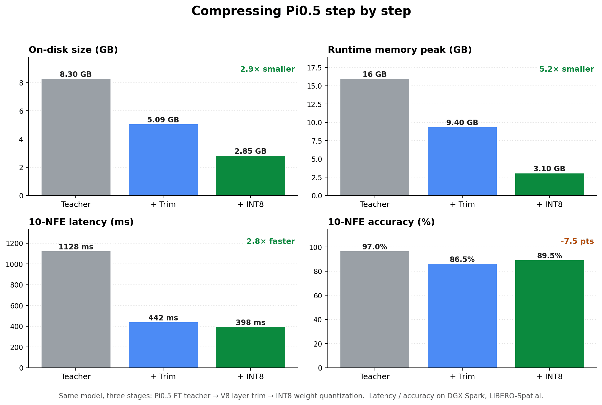
Here's the teacher, then each size-compression step applied in order. Same benchmark and hardware throughout (LIBERO-Spatial on a DGX Spark with a GB10 Blackwell), so the columns are directly comparable:
Note: this week's trim student was distilled from the bf16 FT teacher directly, not from last week's SnapFlow student. We wanted a clean read on what layer pruning costs, without confounding it with an already-modified base model. Composing the two is on the next-week list.
| Pi0.5 FT teacher | + V8 trim size | + int8wo | vs teacher | |
|---|---|---|---|---|
| Params | 4.14 B | 2.31 B | 2.31 B | 1.8× smaller |
| On-disk size | 8.3 GB | 5.09 GB | 2.85 GB | 2.9× smaller |
| Runtime memory peak | ~16 GB | 9.4 GB | 3.1 GB | 5.2× lighter |
| 10-NFE accuracy | ~97% (n=20 only) | 86.5% | 89.5% | −7.5 pts |
| 10-NFE latency | 1128 ms | 442 ms | 398 ms | 2.8× faster |
The compressed model needs about a fifth of the runtime memory, runs nearly 3× faster, and gives up roughly 7 percentage points of accuracy. Whether that tradeoff is worth it depends on your robot, but the main point is: this model now fits on commodity edge accelerators with 4 GB of memory, where the teacher needed a workstation-class GPU.
The pipeline tax
Every combination of base model, compression recipe, training cluster, and target hardware is its own snowflake. Here's what ours looked like.
The paper gives you the recipe. It doesn't tell you what running that recipe end-to-end actually costs across your particular stack: your training cluster, your scheduler, your eval harness, your target hardware. Every (base model × recipe × cluster × deployment target) tuple has its own friction map. Most of that friction shows up as silent failures: the loader succeeds, the script exits zero, the dashboard looks fine, and you only notice when eval drops.
Here's what one tuple cost us this week (Pi0.5 + Shallow-π trim + 8× A100 + DGX Spark + Jetson Orin Nano). Yours will be different. The point of the list isn't the specific six; it's that there is always a six, and someone has to own it.
1. LeRobot's --resume=true silently rebuilds the LR schedule. A resumed run is a fresh schedule, not a continuation. Cost: ~1 day of A100 compute + 1 day to diagnose. Patched locally, issue filed with the maintainers.
2. Pi0.5's from_pretrained ignores saved layer counts. Loads silently broken: 6 trained layers + 12 randomly-initialized ones, no warning from the loader. Cost: ~1.5 hours across two machines. Fix is a re-slicing hook before the state-dict loads.
3. Safetensors and torchao don't round-trip. Safetensors strips torchao's per-channel scales; INT8 weights look right on reload but accuracy is wrong. Cost: ~2 hours. Use torch.save until one side fixes the protocol; “redistribute a quantized VLA” is not a solved problem.
4. Per-step training metrics: enable wandb up front, or they're gone. lerobot's tqdm bar has no numerical data, and we inherited a run config with wandb's run_id: None. Cost: the V3-vs-V8 training curves are gone forever.
5. Multi-machine choreography is its own job. A100 trains, Spark evals, Jetson Orin Nano is the deploy target. Three filesystems, three Python environments, manual scp. State drifts; “where is the latest V8 30k?” is a daily question. Cost: ~30 min/day, compounding across weeks. The real value of a managed pipeline is owning storage, naming, and handoffs, not the model surgery.
6. HuggingFace returns 401 on PaliGemma's config. Auth flaps for gated-but-public configs. Fix: pre-cache locally, set HF_HUB_OFFLINE=1. Cost: ~1 hour first time, zero after. In production, this is an availability bug for a robot fleet at deploy time.
None are dealbreakers individually. But change one variable in the tuple. Swap Pi0.5 for OpenVLA, swap Shallow-π for LayerDrop, swap A100 for H100, swap Orin Nano for Thor. You don't get the same six. You get a different six. The published recipe is shared; the friction map is the snowflake, and it's where the time actually goes. Building and owning that meta-layer, the part that internalizes whichever snowflake you have, is what a managed compression pipeline buys.
What's next
Three open threads:
- Compose time + size distillation. Distill the V8 trim on top of the SnapFlow base, not the raw teacher.
- Graduate quantization from weight-only to W8A8 + calibration for true INT8 GEMM speed.
- Close the absolute-accuracy gap to Shallow-π (94.6% paper L=6 vs our 88.0% at 30k; authors contacted).
Most of all: this week closed the “fits a real robot's budget” gate. The next post covers the deployment.
We are talking to teams running open VLAs in production who want a pipeline like this reliably available as a service. If you have a Pi0, Pi0.5, or OpenVLA setup that runs on an A100 and falls over on your robot, get in touch. Same goes for teams who want a custom fine-tune-distill-quantize pipeline that retriggers automatically when the next SOTA model lands.
Reach out via email or X. The deployment work is in progress now; a real target embodiment to validate against would be the highest-leverage feedback we could get.
Thanks again to Physical Intelligence (Pi0.5), Samsung Research (Shallow-π), Feng et al. (Align-KD), HuggingFace (LeRobot), and the PyTorch team (torchao). This week was 90% standing on other people's shoulders.